plot_cosinor¶

Summary¶

plot_cosinor fits and draws a single-component cosinor rhythm for one value column over cyclic time. It plots per-timepoint mean plus SEM points and one fitted cosine curve per group.

Registry name: cosinor.

Example figure¶

plot_cosinor example figure

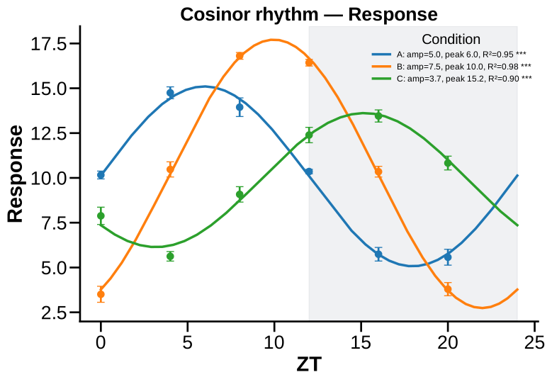
24 h cosinor fits for three groups with distinct acrophase and amplitude. Rendered from the synthetic example dataset.

Signature¶

plot_cosinor(
    experiment,
    column,
    time_col="Time",
    group_col=None,
    period=24.0,
    period_free=False,
    specificity=None,
    filter_by=None,
    time_map=None,
    palette=None,
    show_points=True,
    night_shade="auto",
    title=None,
    save=True,
    save_path=None,
    save_name=None,
    subfolder=None,
    montage=False,
    dpi=600,
    return_data=False,
)

Input Object Types¶

Object type	Accepted?	Notes
`Batch`	Yes	Uses `batch.summary`.
`Experiment`	Yes	Uses `experiment.summary`.
`MiniExperiment`	Yes	Works when its summary contains the needed time and value columns.
`pandas.DataFrame`	Yes	Used directly as the subject-level frame.

Parameters¶

Parameter	Type	Default	Meaning
`experiment`	PyFLASH-like object or `DataFrame`	required	Source with a subject-level summary table.
`column`	`str`	required	Numeric measurement to fit.
`time_col`	`str`	`"Time"`	Time column. Numeric values, mapped labels, and trailing digits are supported.
`group_col`	`str` or `None`	`None`	Group column. If omitted or missing, all rows are fit as one group.
`period`	number	`24.0`	Cycle length in the same units as `time_col`.
`period_free`	`bool`	`False`	Fit period as a parameter instead of fixing it.
`filter_by`	dict, tuple, list, or `None`	`None`	Preferred row filter. Lists run queue mode.
`time_map`	`dict` or `None`	`None`	Map time labels to numeric values, for example `{"ZT0": 0, "ZT6": 6}`.
`palette`	palette, dict, or `None`	`None`	Group colour palette or mapping.
`show_points`	`bool`	`True`	Show per-timepoint mean plus SEM points.
`night_shade`	`"auto"`, tuple, or false-like	`"auto"`	Shade a night interval. `"auto"` shades 12 to 24 for a 24-hour period.
`title`	`str` or `None`	`None`	Figure title.
`save`	`bool`	`True`	Save the figure.
`save_path`	Path-like or `None`	`None`	Base output folder override.
`save_name`	`str` or `None`	`None`	File stem override. Default is `<column>_cosinor`.
`subfolder`	`str` or `None`	`None`	Optional subfolder passed to the save helper.
`montage`	`bool`	`False`	Mark saved figure for montage collection when a pipeline has armed montage capture.
`dpi`	`int`	`600`	Save DPI.
`return_data`	`bool`	`False`	Return fit dictionaries with the figure.

Returns¶

Return value	Type	Meaning
`fig`	`matplotlib.figure.Figure`	Returned by default.
`(fig, fits)`	tuple	Returned when `return_data=True`. `fits` maps group name to a fit dictionary, or `None` for failed group fits.
`result`	`dict`	Queue mode returns a dictionary keyed by filter value.

Each successful fit dictionary comes from fit_cosinor and includes period, mesor, amplitude, acrophase, r_squared, p, p_rhythm, n, and a predict callable.

Saved Outputs¶

With save=True, the figure is saved through save_fig() to either save_path or the source object's standard figure folder. The default file stem is:

<column>_cosinor

The function also emits a structured rhythm record through the describe/report layer when that layer is active.

Examples¶

Fit a 24-hour rhythm from a Batch¶

from PyFLASH.plotting import plot_cosinor

fig, fits = plot_cosinor(
    batch,
    column="GFAP_IntDen",
    time_col="ZT",
    group_col="Diagnosis",
    period=24,
    save=False,
    return_data=True,
)

print(fits["Control"]["acrophase"])

Use explicit time mapping¶

plot_cosinor(
    batch.summary,
    column="Activity",
    time_col="Time",
    group_col="Genotype",
    time_map={"ZT0": 0, "ZT6": 6, "ZT12": 12, "ZT18": 18},
    save=False,
)

Queue filters¶

figures = plot_cosinor(
    batch,
    column="GFAP_IntDen",
    filter_by=[{"Sex": "Female"}, {"Sex": "Male"}],
    group_col="Diagnosis",
    save=False,
)

print(figures.keys())

Notes¶

The function raises ValueError when column or time_col is missing, or when no numeric time/value rows remain.
fit_cosinor requires at least four finite time/value points per group. Group-level fit failures are logged and shown in the legend.
The legend reports amplitude, peak/acrophase, R squared, and a rhythmicity marker based on the zero-amplitude F-test.
period_free=True fits a free-running period and is useful for multi-cycle data. Keep fixed-period and free-period plots labelled clearly.
Clock labels such as ZT0 are converted with time_map first, then numeric conversion, then trailing digits.