plot_timecourse
Summary
plot_timecourse fits and draws a growth curve per group across an ordered time
variable. It is registered as timecourse.
Use it for subject-level summaries measured across ordered weeks, months, ages, or other time-like factors.
Example figure
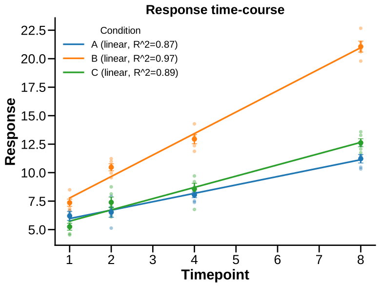
Longitudinal growth curves per group across timepoints. Rendered from the synthetic example dataset.
Signature
plot_timecourse(batch, column, time_col='Time', group_col='Genotype', model='auto', specificity=None, filter_by=None, time_map=None, animal_col='AnimalName', subject_col=None, palette=None, show_points=True, title=None, save=False, save_path=None, save_name=None, dpi=600, return_data=False, condition_col='Condition', factor_cols=None, group_list=None, groups=None, group_cols=None, dataframe_kwargs=None)
Input Object Types
| Object type | Accepted? | Notes |
|---|---|---|
Batch |
Yes | Main supported input. Reads batch.summary. |
Experiment |
Yes | Works when it exposes a non-empty .summary. |
MiniExperiment |
Yes | Works for summary-style data. |
pandas.DataFrame |
Yes | Wrapped internally; pass group_col and subject_col when needed. |
Parameters
| Parameter | Type | Default | Meaning |
|---|---|---|---|
batch |
Batch, experiment-like object, or DataFrame |
required | Data source containing a summary table. |
column |
string | required | Numeric response column to fit and plot. |
time_col |
string | 'Time' |
Column containing time labels or values. |
group_col |
string | 'Genotype' |
Column whose levels get separate curves. |
model |
string | 'auto' |
Accepted values: 'auto', 'linear', 'exponential', or 'logistic'. |
filter_by / specificity |
mapping, tuple, list, or None |
None |
Row filter before fitting. |
time_map |
mapping or None |
None |
Maps categorical labels to numeric time values, e.g. {"WeekTwo": 2}. |
subject_col / animal_col |
string or None |
None, 'AnimalName' |
Subject column for raw DataFrame adaptation. animal_col is the legacy alias. |
palette |
dict or None |
None |
Optional color map for group levels. |
show_points |
bool | True |
Show individual points behind mean +/- SEM summaries. |
title |
string or None |
None |
Custom title. |
save, save_path, save_name, dpi |
saving options | False, None, None, 600 |
Figure saving controls. |
return_data |
bool | False |
Return fit dictionaries with the figure. |
Returns
| Return value | Type | Meaning |
|---|---|---|
fig |
matplotlib.figure.Figure |
Timecourse figure. |
(fig, fits) |
tuple | Returned when return_data=True. |
fits |
dict |
Group name to fit dictionary, or None if fitting failed for that group. |
Fit dictionaries come from PyFLASH.stats_extra.fit_growth_curve and include
model, params, r_squared, aic, n, predict, and all_models.
Saved Outputs
save=False by default. With save=True, PyFLASH writes an SVG figure to
save_path when supplied. Otherwise it uses batch.fig_path, then
batch.data_path, then the current folder.
The default filename stem is <column>_timecourse; pass save_name to
override it.
Examples
Minimal timecourse:
from PyFLASH.plotting import plot_timecourse

fig = plot_timecourse(
    batch,
    "Abeta_Count",
    time_col="Time",
    group_col="Genotype",
)
Categorical time labels with returned fits:
fig, fits = plot_timecourse(
    df,
    "Abeta_Count",
    time_col="Week",
    group_col="Genotype",
    subject_col="AnimalName",
    time_map={"WeekTwo": 2, "WeekFour": 4, "WeekEight": 8},
    model="auto",
    return_data=True,
)
Reuse a fitted curve:
fit = fits["hAPP"]
times = [2, 4, 8]
predict = fit["predict"]
predicted = predict(times)
print(fit["model"], fit["r_squared"], predicted)
Notes
Time values are resolved in this order: explicit time_map, numeric coercion,
then trailing digits from string labels. Pass time_map when labels do not have
usable numeric content.
model="auto" chooses among linear, exponential, and logistic candidates by
AIC when enough data are available. Logistic fits require positive time values.
The plot shows individual points and per-timepoint mean +/- SEM summaries; the
fit itself is computed from all finite (time, value) rows in each group.
This registry entry is currently describe-layer unreviewed; use
return_data=True for machine-readable fit details.