plot_power_curve¶

Summary¶

plot_power_curve draws statistical power as sample size changes. It is registered as power_curve.

Use it to compare assumed standardized effect sizes against per-group sample sizes before or after an experiment. The optional batch argument is used only to resolve a save folder.

Example figure¶

plot_power_curve example figure

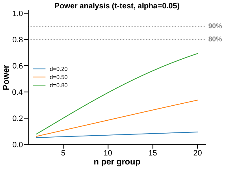
Statistical power vs n per group for effect sizes 0.2 / 0.5 / 0.8. Rendered from the synthetic example dataset.

Signature¶

plot_power_curve(batch=None, *, effect_sizes=(0.2, 0.5, 0.8), n_range=(2, 30), alpha=0.05, observed=None, observed_n=None, target_powers=(0.8, 0.9), test='t-test', k_groups=2, title=None, save=False, save_path=None, save_name='power_curve', dpi=600, return_data=False)

Input Object Types¶

Object type	Accepted?	Notes
`Batch`	Optional	Used only to resolve `fig_path` or `data_path` when saving.
`Experiment`	Optional	Also works as a save-path holder if it has `fig_path` or `data_path`.
`MiniExperiment`	Optional	Same as above.
`pandas.DataFrame`	Not needed	The function does not inspect table contents.

Parameters¶

Parameter	Type	Default	Meaning
`batch`	object or `None`	`None`	Optional object used for save-path resolution.
`effect_sizes`	sequence of floats	`(0.2, 0.5, 0.8)`	Standardized effects to plot.
`n_range`	`(int, int)`	`(2, 30)`	Inclusive per-group sample-size range.
`alpha`	float	`0.05`	Significance threshold used in power calculations.
`observed`	float or `None`	`None`	Optional observed effect size to add as a highlighted curve.
`observed_n`	int or `None`	`None`	Optional vertical reference line for observed per-group sample size.
`target_powers`	sequence of floats	`(0.8, 0.9)`	Horizontal guide lines.
`test`	string	`'t-test'`	Accepted values include `'t-test'` and `'anova'`/`'f'`/`'f-test'`.
`k_groups`	int	`2`	Number of groups for ANOVA power.
`title`	string or `None`	`None`	Custom title.
`save`, `save_path`, `save_name`, `dpi`	saving options	`False`, `None`, `'power_curve'`, `600`	Figure saving controls.
`return_data`	bool	`False`	Return the computed power table with the figure.

Returns¶

Return value	Type	Meaning
`fig`	`matplotlib.figure.Figure`	Power curve figure.
`(fig, data)`	tuple	Returned when `return_data=True`.
`data`	`pandas.DataFrame`	Columns: `effect_size`, `n_per_group`, `power`, and `observed`.

Saved Outputs¶

save=False by default. With save=True, PyFLASH writes an SVG figure to save_path when supplied. Otherwise it uses batch.fig_path, then batch.data_path, then the current folder.

The default filename stem is power_curve; pass save_name to override it.

Examples¶

Minimal t-test power curves:

from PyFLASH.plotting import plot_power_curve

fig = plot_power_curve(
    effect_sizes=(0.5, 0.8),
    n_range=(4, 20),
)

Include an observed effect and inspect the table:

fig, data = plot_power_curve(
    effect_sizes=(0.3, 0.5, 0.8),
    n_range=(3, 25),
    observed=0.62,
    observed_n=8,
    return_data=True,
)

near_80 = data[data["power"] >= 0.8].groupby("effect_size").first()
print(near_80[["n_per_group", "power"]])

ANOVA power:

fig = plot_power_curve(
    effect_sizes=(0.25, 0.4),
    n_range=(5, 30),
    test="anova",
    k_groups=3,
)

Notes¶

For test="t-test", PyFLASH uses statsmodels.stats.power.TTestIndPower with equal group sizes. For ANOVA, it uses FTestAnovaPower with total observations computed as n_per_group * k_groups.

Power curves depend on assumed standardized effect sizes. Treat them as design diagnostics, not as evidence that any specific marker is significant.

This registry entry is describe-layer exempt because it is a design diagnostic rather than a data-derived inferential result.